Logistic regression and implementation#
1. Math background#
1.1 Exponential family distribution#
The general form of an exponential family distribution is:
In the context of generalized linear models (GLMs), the natural parameter \(\eta\) is linked to the predictors \(\mathbf{x}\) via:
Thus, the conditional density of \(y\) given \(\mathbf{x}\) becomes:
The logistic regression Exponential family distribution for logistic regression: Now, we rewrite Bernoulli distribution in terms of exponential family distribution:
where,
In logistic regression, we assume \(\eta = \boldsymbol{x}^T_i\beta\), so
1.2 Maximax likehood estimation#
where \(y\) is the total number of success in \(n\) trials.
The corresponding log-likelihood is
1.2.1. Gradient#
Take first-order derivative of \(\ell(\mathbf{y}|\mathbf{X},\boldsymbol{\beta})\) about \(\boldsymbol{\beta}\), we have
where,
1.2.2. Hessian (second derivative matrix)#
Given \(p_i = {(1+ e^{-\boldsymbol{x}_i\boldsymbol{\beta}})}^{-1}\) and \(e^{\boldsymbol{x}_i\boldsymbol{\beta}} = \frac{p_i}{1-p_i}\), then
Where, \(\mathbf{W} = diag[p_i(1-p_i)]\).
1.3 Numerical Approximation#
1.3.1 Gradient Ascent (on log-likelihood)#
We aim to maximize the log-likelihood:
Or simplified:
Update rule:
Where:
\(\alpha\): learning rate
\(\boldsymbol{\mu} = \sigma(\mathbf{X} \boldsymbol{\beta}^{(t)})\)
This is a first-order method.
1.3.2. Newton-Raphson (Second-order method)#
Use both the gradient and the Hessian to update \(\boldsymbol{\beta}\):
Gradient:
Hessian:
Update rule:
Or equivalently:
This method converges faster than gradient ascent but requires inverting a matrix, which can be expensive.
1.3.3. Iteratively Reweighted Least Squares (IRLS)#
IRLS is a special case of Newton-Raphson, reformulated as a weighted least squares:
Define:
Pseudo-response (working response):
\[ \mathbf{z} = \boldsymbol{\eta} + \frac{\mathbf{y} - \boldsymbol{\mu}}{\mu_i (1 - \mu_i)} \]Weight matrix:
\[ \mathbf{W} = \operatorname{diag}(\mu_i (1 - \mu_i)) \]
Solve at each step:
This looks like a weighted linear regression, where weights and pseudo-response ( \mathbf{z} ) are updated at each iteration.
1.3.4 Summary Comparison#
Method |
Uses |
Update Formula |
Notes |
|---|---|---|---|
Gradient Ascent |
Gradient only |
\(\boldsymbol{\beta}^{(t+1)} = \boldsymbol{\beta}^{(t)} + \alpha \mathbf{X}^T (\mathbf{y} - \boldsymbol{\mu})\) |
Simple, slow, needs tuning \(\alpha\) |
Newton-Raphson |
Gradient + Hessian |
\(\boldsymbol{\beta}^{(t+1)} = \boldsymbol{\beta}^{(t)} + (\mathbf{X}^T \mathbf{W} \mathbf{X})^{-1} \mathbf{X}^T (\mathbf{y} - \boldsymbol{\mu})\) |
Faster convergence, more computation |
IRLS |
Weighted Least Squares |
\(\boldsymbol{\beta}^{(t+1)} = (\mathbf{X}^T \mathbf{W} \mathbf{X})^{-1} \mathbf{X}^T \mathbf{W} \mathbf{z}\) |
Very popular for GLMs |
1.5 Implementation#
1.5.1 Simulate dataset#
import numpy as np
import torch
from torch.nn.functional import sigmoid
from sklearn.linear_model import LogisticRegression
from sklearn.metrics import accuracy_score
import time

# Setup
device = torch.device("cpu")
np.random.seed(42)

# Parameters
n_samples = 500
n_features = 10

# Simulate features and labels
X_np = np.random.randn(n_samples, n_features)
true_beta = np.random.randn(n_features)
logits = X_np @ true_beta
probs = 1 / (1 + np.exp(-logits))
y_np = np.random.binomial(1, probs)

# Convert to PyTorch
X = torch.tensor(X_np, dtype=torch.float32, device=device)
y = torch.tensor(y_np, dtype=torch.float32, device=device).view(-1, 1)
1.5.2. Accuracy Helper Function (Code Cell)#
def compute_accuracy(beta, X, y):
    with torch.no_grad():
        preds = (sigmoid(X @ beta) >= 0.5).float()
        return (preds == y).float().mean().item()
1.5.3. Gradient Ascent (Code Cell)#
def gradient_ascent(X, y, lr=0.1, max_iter=100):
    # Initialize beta (weights) as a zero vector with shape (features, 1)
    # requires_grad=True allows autograd to track operations on beta
    beta = torch.zeros((X.shape[1], 1), requires_grad=True, device=device)

    # Iterate for a fixed number of steps
    for _ in range(max_iter):
        # Compute the predicted probabilities using the sigmoid function
        mu = sigmoid(X @ beta)

        # Compute the negative log-likelihood loss
        # Add small epsilon (1e-8) to avoid log(0) instability
        loss = -torch.mean(y * torch.log(mu + 1e-8) + (1 - y) * torch.log(1 - mu + 1e-8))

        # Compute gradients via backpropagation
        loss.backward()

        # Update beta using gradient ascent
        with torch.no_grad():
            # Gradient ascent step: move in the direction of the negative gradient
            beta += lr * (-beta.grad)

            # Reset gradients to zero for the next iteration
            beta.grad.zero_()

    # Detach the tensor from the computation graph and return it
    return beta.detach()
1.5.4. Newton-Raphson (Code Cell)#
def newton_raphson(X, y, max_iter=10):
    # Initialize beta (weights) as zeros; shape = (features, 1)
    beta = torch.zeros((X.shape[1], 1), device=device)

    # Loop for a fixed number of iterations
    for _ in range(max_iter):
        # Compute the predicted probabilities using the sigmoid function
        mu = sigmoid(X @ beta)  # shape: (n_samples, 1)

        # Compute the diagonal weight matrix W = diag(mu * (1 - mu))
        W = torch.diag((mu * (1 - mu)).flatten())  # shape: (n_samples, n_samples)

        # Compute the adjusted response z (working variable in IRLS/NR)
        # z = η + (y - μ) / W = η + W⁻¹ (y - μ)
        # η = X @ β
        z = X @ beta + torch.inverse(W + 1e-4 * torch.eye(W.shape[0])) @ (y - mu)

        # Update rule for Newton-Raphson:
        # β = (Xᵀ W X)⁻¹ Xᵀ W z
        # Add a small ridge term (1e-4 * I) for numerical stability
        beta = torch.inverse(X.T @ W @ X + 1e-4 * torch.eye(X.shape[1])) @ X.T @ W @ z

    # Return final estimate of beta
    return beta
1.5.5. IRLS (Code Cell)#
def irls(X, y, max_iter=10):
    # Initialize beta (weights) as zeros; shape = (features, 1)
    beta = torch.zeros((X.shape[1], 1), device=device)

    # Iteratively update beta using weighted least squares
    for _ in range(max_iter):
        # Compute the linear predictor η = X @ beta
        eta = X @ beta

        # Compute predicted probabilities using sigmoid(η)
        mu = sigmoid(eta)  # shape: (n_samples, 1)

        # Compute weights: W_diag = μ(1 - μ) (flattened for diag)
        W_diag = (mu * (1 - mu)).flatten()  # shape: (n_samples,)

        # Construct the diagonal weight matrix W
        W = torch.diag(W_diag)  # shape: (n_samples, n_samples)

        # Compute the working response z:
        # z = η + (y - μ) / [μ(1 - μ)]
        z = eta + (y - mu) / (W_diag.view(-1, 1) + 1e-8)  # add epsilon for numerical stability

        # Weighted least squares update:
        # β = (Xᵀ W X)⁻¹ Xᵀ W z
        beta = torch.inverse(X.T @ W @ X + 1e-4 * torch.eye(X.shape[1])) @ X.T @ W @ z

    # Return the final estimate of beta
    return beta
1.5.6. Compare All Methods (Code Cell)#
results = {}

start = time.time()
beta_gd = gradient_ascent(X, y)
results['Gradient Ascent'] = (time.time() - start, compute_accuracy(beta_gd, X, y))

start = time.time()
beta_nr = newton_raphson(X, y)
results['Newton-Raphson'] = (time.time() - start, compute_accuracy(beta_nr, X, y))

start = time.time()
beta_irls = irls(X, y)
results['IRLS'] = (time.time() - start, compute_accuracy(beta_irls, X, y))

# Scikit-learn
sk_model = LogisticRegression(fit_intercept=False, max_iter=1000)
start = time.time()
sk_model.fit(X_np, y_np)
sk_time = time.time() - start
sk_acc = accuracy_score(y_np, sk_model.predict(X_np))
results['scikit-learn'] = (sk_time, sk_acc)

# Print comparison
import pandas as pd
pd.DataFrame(results, index=['Time (s)', 'Accuracy']).T
| Time (s) | Accuracy | |
|---|---|---|
| Gradient Ascent | 0.012920 | 0.834 |
| Newton-Raphson | 0.016865 | 0.836 |
| IRLS | 0.001456 | 0.836 |
| scikit-learn | 0.001023 | 0.836 |
1.5.7. Plot Gradient Ascent Convergence (Optional Code Cell)#
import matplotlib.pyplot as plt
import numpy as np
import torch
from torch.nn.functional import sigmoid
from sklearn.linear_model import LogisticRegression
# --------- Gradient Ascent with loss tracking ---------
def gradient_ascent_trace(X, y, lr=0.1, max_iter=100):
# Initialize beta with zeros and enable gradient tracking
beta = torch.zeros((X.shape[1], 1), requires_grad=True, device=device)
loss_trace = [] # Store loss values for plotting
for _ in range(max_iter):
# Predicted probabilities using sigmoid function
mu = sigmoid(X @ beta)
# Compute negative log-likelihood (add small epsilon for numerical stability)
loss = -torch.mean(y * torch.log(mu + 1e-8) + (1 - y) * torch.log(1 - mu + 1e-8))
loss_trace.append(loss.item()) # Store current loss
# Compute gradient
loss.backward()
# Gradient ascent step
with torch.no_grad():
beta += lr * (-beta.grad) # Ascend the negative gradient
beta.grad.zero_() # Reset gradients for next iteration
return beta.detach(), loss_trace # Return final beta and loss history
# --------- Newton-Raphson with loss tracking ---------
def newton_raphson_trace(X, y, max_iter=10):
beta = torch.zeros((X.shape[1], 1), device=device)
loss_trace = []
for _ in range(max_iter):
mu = sigmoid(X @ beta) # Predicted probabilities
loss = -torch.mean(y * torch.log(mu + 1e-8) + (1 - y) * torch.log(1 - mu + 1e-8))
loss_trace.append(loss.item())
# Construct weight matrix W = diag(mu * (1 - mu))
W = torch.diag((mu * (1 - mu)).flatten())
# Compute pseudo-response z
z = X @ beta + torch.inverse(W + 1e-4 * torch.eye(W.shape[0])) @ (y - mu)
# Newton-Raphson update: beta = (Xᵀ W X)⁻¹ Xᵀ W z
beta = torch.inverse(X.T @ W @ X + 1e-4 * torch.eye(X.shape[1])) @ X.T @ W @ z
return beta, loss_trace
# --------- IRLS with loss tracking ---------
def irls_trace(X, y, max_iter=10):
beta = torch.zeros((X.shape[1], 1), device=device)
loss_trace = []
for _ in range(max_iter):
eta = X @ beta # Linear predictor
mu = sigmoid(eta) # Predicted probabilities
loss = -torch.mean(y * torch.log(mu + 1e-8) + (1 - y) * torch.log(1 - mu + 1e-8))
loss_trace.append(loss.item())
W_diag = (mu * (1 - mu)).flatten() # Diagonal of weight matrix
W = torch.diag(W_diag) # Weight matrix W
# Compute pseudo-response z
z = eta + (y - mu) / (W_diag.view(-1, 1) + 1e-8) # Add epsilon to prevent div-by-zero
# IRLS update: beta = (Xᵀ W X)⁻¹ Xᵀ W z
beta = torch.inverse(X.T @ W @ X + 1e-4 * torch.eye(X.shape[1])) @ X.T @ W @ z
return beta, loss_trace
# --------- scikit-learn model as benchmark ---------
# Fit logistic regression using sklearn for reference
sk_model = LogisticRegression(fit_intercept=False, max_iter=1000)
sk_model.fit(X_np, y_np)
# Compute loss using sklearn's fitted coefficients
logits_sk = X_np @ sk_model.coef_.flatten()
mu_sk = 1 / (1 + np.exp(-logits_sk))
loss_sklearn = -np.mean(y_np * np.log(mu_sk + 1e-8) + (1 - y_np) * np.log(1 - mu_sk + 1e-8))
# --------- Run all methods and collect loss traces ---------
_, loss_gd = gradient_ascent_trace(X, y, lr=0.1, max_iter=100)
_, loss_nr = newton_raphson_trace(X, y, max_iter=10)
_, loss_irls = irls_trace(X, y, max_iter=10)
# For sklearn, use a flat horizontal line for loss comparison
loss_sklearn_line = [loss_sklearn] * max(len(loss_gd), len(loss_nr), len(loss_irls))
# --------- Plot convergence of all methods ---------
plt.figure(figsize=(10, 6))
# Gradient Ascent: smooth line
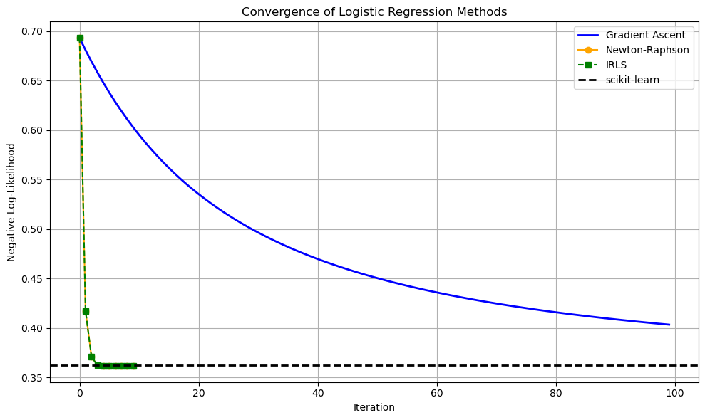
plt.plot(loss_gd, label="Gradient Ascent", color="blue", linewidth=2)
# Newton-Raphson: dots with orange line
plt.plot(np.arange(len(loss_nr)), loss_nr, 'o-', label="Newton-Raphson", color="orange", markersize=6)
# IRLS: green dashed line with squares
plt.plot(np.arange(len(loss_irls)), loss_irls, 's--', label="IRLS", color="green", markersize=6)
# scikit-learn: black dashed horizontal line
plt.axhline(loss_sklearn, color="black", linestyle="--", linewidth=2, label="scikit-learn")
# Decorate the plot
plt.xlabel("Iteration")
plt.ylabel("Negative Log-Likelihood")
plt.title("Convergence of Logistic Regression Methods")
plt.legend()
plt.grid(True)
plt.tight_layout()
plt.show()