Diagnose scale issue of summary statistics

suppressPackageStartupMessages(library(tidyverse))
library(data.table)
library(ggplot2)
library(patchwork)

In an association of a single SNP \(j\), we have a simple linear model (Yang, Jian, et al(2012)):

\[\begin{equation}y = X_jb_j + e \tag{1}\end{equation}\]

Based on OLS, we have

\[\begin{equation}\hat{b}_j = (X_j^TX_j)^{-1}X_j^Ty = D_j^{-1}X_j^Ty\tag{2}\end{equation}\]

and

\[\begin{equation}\sigma_b^2 = \sigma_e^2 (X_j^TX_j)^{-1} = \sigma_e^2D_j^{-1}\tag{3}\end{equation}\]

Based on ANOVA, we have

\[\begin{equation}\sigma_e^2 = \frac{y^Ty - \hat{y}^T\hat{y}}{(n-1)} = \frac{y^Ty - (X_j\hat{b}_j)^T(X_j\hat{b}_j)}{(n-1)} \tag{4}\end{equation}\]

Based on probability, we have Z-score

\[\begin{equation}z_j = \frac{\hat{b}_j}{\sigma_b}\tag{5}\end{equation}\]

Reformatting Eq(4), we derive

\[\begin{equation}(n-1)\sigma_e^2 = y^Ty - \hat{b}_j^2D_j \tag{6}\end{equation}\]

By combining Eq(3) and Eq(5) into Eq(6), we have

\[\begin{split} \begin{equation} \begin{aligned}(n-1)\sigma_b^2D_j &= y^Ty - z_j^2\sigma_b^2D_j \\ \Leftrightarrow \sigma_b &= \sqrt{\frac{y^Ty}{(n-1)D_j+z_j^2D_j}}\end{aligned} \tag\end{equation}{7} \end{equation} \end{split}\]

Here, we assume trait phenotype \(y\) is standardized (thus, \(y^Ty = n\)) and \(D_j = 2p_j(1-p_j)n\). If only summary statistics Z score is provided, we can re-estimate \(\hat{b}_j\) and \(\sigma_b\) given allele frequency \(p\), sample size \(n\) and zscore \(z\), therefore,

\[\begin{split} \begin{equation} \begin{aligned}\sigma_b &= \sqrt{\frac{n}{(n-1)2p_j(1-p_j)n+z_j^22p_j(1-p_j)n}} \\ &= \sqrt{\frac{1}{(n-1)2p_j(1-p_j)+z_j^22p_j(1-p_j)}}\end{aligned}\tag{8} \end{equation} \end{split}\]

Also, we have

\[\begin{equation}b_j = \sqrt{\frac{z^2}{(n-1)2p_j(1-p_j)+z_j^22p_j(1-p_j)}}\tag{9}\end{equation}\]

############################################
### Run a simulation to simulate gene exression
### y = beta * x + e, where y is scaled gene expression
### x is the genotype at 0/1/2 scale, BETA and SE
###  is the original effect size and standard error
###  N is the sample size
###  A1Freq is the allele frequency 
###  zz is the zscore
############################################
set.seed(1234)
sumPath = "~/Documents/personal/SbayesAnno/downSampling/Verify0319/summary/"
smrIndFileSuffix = "ukbg-chr22-causal-model-50k-ind"
geneLDFile = paste0(sumPath,smrIndFileSuffix)
xqtl = fread(paste0(geneLDFile,".q.query.gz"))
test = xqtl %>% mutate(zz = BETA/SE) %>%
mutate(beta = zz / sqrt(2 * A1Freq * (1-A1Freq) * (N-1 + zz^2)),
       betaScale = BETA * sqrt(2 * A1Freq * (1-A1Freq)),
se = 1 / sqrt(2 * A1Freq * (1-A1Freq) * (N-1 + zz^2))
) 
head(test)
options(repr.plot.width = 12, repr.plot.height = 6)
#### beta based on zscore and Original beta
p1 = ggplot(test, aes(x = beta, y = BETA,)) +
  geom_point() +
  geom_abline(intercept = 0, slope = 1, linetype = "dashed", color = "red") +
  labs(
    y = "Orignal Beta",
    x = "Beta based on Zscore",
    title = "Fig 1.1 Orignal Beta vs Beta based on Zscore in the simulation"
  ) + theme_minimal();
  #### beta based on zscore and Original beta
p2 = ggplot(test, aes(x = beta, y = betaScale)) +
  geom_point() +
  geom_abline(intercept = 0, slope = 1, linetype = "dashed", color = "red") +
  labs(
    x = "Beta based on Zscore",
    y = "scaled Beta",
    title = "Fig 1.2 scaled Beta vs Beta based on Zscore in the simulation"
  ) + theme_minimal();
(p1 + p2) 
print(paste0("correlation between beta and BETA is ", cor(test$beta, test$BETA)))
print(paste0("correlation between beta and betaScale is ", cor(test$beta, test$betaScale)))

A data.table: 6 x 18

GeneID	GeneChr	GeneLength	GenePhyPos	SNPID	SNPChr	SNPPhyPos	A1	A2	A1Freq	BETA	SE	Pvalue	N	zz	beta	betaScale	se
<chr>	<int>	<int>	<dbl>	<chr>	<int>	<int>	<chr>	<chr>	<dbl>	<dbl>	<dbl>	<dbl>	<int>	<dbl>	<dbl>	<dbl>	<dbl>
ENSG00000187905	22	-999	21409346	rs428214	22	21361060	T	G	0.155100	-0.006123455	0.008735706	4.833227e-01	50000	-0.7009685	-0.006123393	-0.003134874	0.008735618
ENSG00000187905	22	-999	21409346	rs373092	22	21361870	G	T	0.027860	-0.511740506	0.019078813	2.225000e-308	50000	-26.8224492	-0.511735459	-0.119102192	0.019078625
ENSG00000187905	22	-999	21409346	rs398577	22	21362849	A	C	0.139213	-0.275573105	0.009060138	2.225000e-308	50000	-30.4159945	-0.275319807	-0.134908581	0.009051810
ENSG00000187905	22	-999	21409346	rs2075274	22	21363306	A	G	0.371860	-0.301651835	0.006405235	2.225000e-308	50000	-47.0945754	-0.301531294	-0.206176388	0.006402676
ENSG00000187905	22	-999	21409346	rs2516542	22	21363505	T	C	0.126070	-0.342185229	0.009403473	2.225000e-308	50000	-36.3892402	-0.342181893	-0.160627706	0.009403381
ENSG00000187905	22	-999	21409346	rs2075276	22	21363744	C	T	0.498304	-0.434683323	0.006030275	2.225000e-308	50000	-72.0834933	-0.433913672	-0.307365757	0.006019598

[1] "correlation between beta and BETA is 0.999999335847599"
[1] "correlation between beta and betaScale is 0.957713529698195"

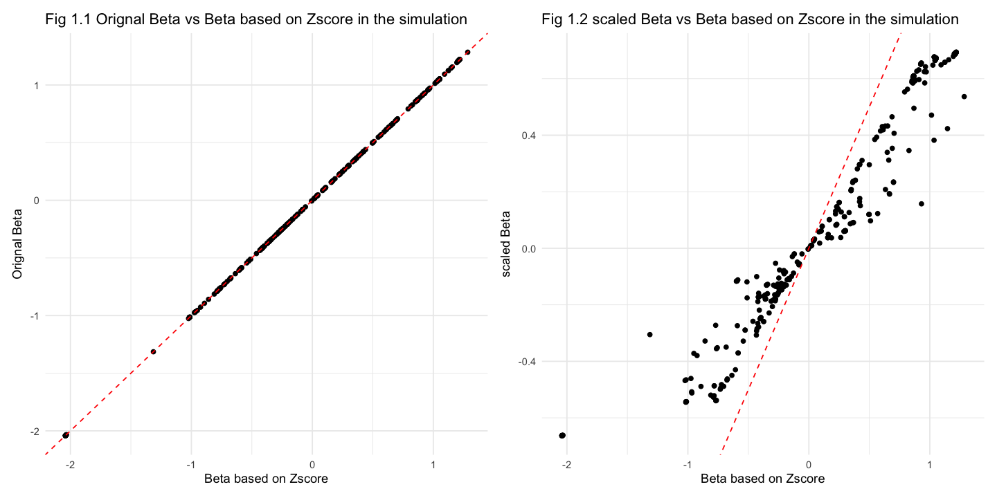
Fig 1.1 suggests that the original beta values are very well captured by the Z-score-based estimates. In Fig 1.2 (right plot), the data points systematically deviate from the reference line \(y = x\), indicating a upward biased (Scaled Beta is larger than Beta based on Z-score).

############################################
### blood pQTLs
############################################
library(data.table)
library(tidyverse)
beqtlPath = "~/Downloads/data/xqtl/"
beqtl = fread(paste0(beqtlPath,"ukb-ppp-pGWAS-v1-eur-hg19-pro3k-chr22-cis1M-HM3q.query.gz"))
test = beqtl %>% mutate(zz = BETA/SE) %>%
mutate(beta = zz / sqrt(2 * A1Freq * (1-A1Freq) * (N-1 + zz^2)),
       betaScale = BETA * sqrt(2 * A1Freq * (1-A1Freq)),
se = 1 / sqrt(2 * A1Freq * (1-A1Freq) * (N-1 + zz^2))
) %>% slice_sample(n = 10000)
head(test)
options(repr.plot.width = 12, repr.plot.height = 6)
p1 = ggplot(test, aes(x = beta, y = BETA)) +
  geom_point() +
  geom_abline(intercept = 0, slope = 1, linetype = "dashed", color = "red") +
  labs(
    y = "Beta from raw data",
    x = "Beta based on Zscore",
    title = "Randomly selected 10,000 SNPs from genes for blood pQTLs"
  ) + theme_minimal()
p2 =  test  %>%
mutate( betaScale = BETA * sqrt(2 * A1Freq * (1-A1Freq))) %>%
 ggplot( aes(x = beta, y = betaScale)) +
  geom_point() +
  geom_abline(intercept = 0, slope = 1, linetype = "dashed", color = "red") +
  labs(
    y = "Fig 2.1 Beta based on Zscore adjusted by snp2pq (beta * sqrt(2 * A1Freq * (1-A1Freq)))",
    x = "Fig 2.2 Beta based on Zscore",
    title = "Randomly selected 10,000 SNPs from genes for blood pQTLs"
  ) + theme_minimal()
  p1 + p2
 print(paste0("correlation between beta and BETA is ", cor(test$beta, test$BETA)))
print(paste0("correlation between beta and betaScale is ", cor(test$beta, test$betaScale)))

A data.table: 6 x 18

GeneID	GeneChr	GeneLength	GenePhyPos	SNPID	SNPChr	SNPPhyPos	A1	A2	A1Freq	BETA	SE	Pvalue	N	zz	beta	betaScale	se
<chr>	<int>	<int>	<dbl>	<chr>	<int>	<int>	<chr>	<chr>	<dbl>	<dbl>	<dbl>	<dbl>	<int>	<dbl>	<dbl>	<dbl>	<dbl>
OID20838_ENSG00000100083	22	-999	37621144	rs86582	22	37603390	T	C	0.194599	0.013366000	0.00972440	0.169292502	32922	1.3744807	0.0135300154	0.0074832945	0.009843729
OID30372_ENSG00000099977	22	-999	23975534	rs17004053	22	24250835	G	A	0.032967	-0.091722200	0.02052610	0.000007875	33924	-4.4685644	-0.0960545088	-0.0231606009	0.021495608
OID30382_ENSG00000100345	22	-999	36334645	rs5999726	22	35502070	A	C	0.620594	0.012363900	0.00778328	0.112168685	33924	1.5885205	0.0125677829	0.0084845022	0.007911628
OID20865_ENSG00000130638	22	-999	45758552	rs1555208	22	46577210	T	G	0.090022	-0.004931240	0.01465610	0.736521511	32922	-0.3364633	-0.0045813734	-0.0019960017	0.013616264
OID30352_ENSG00000100024	22	-999	24511248	rs9608196	22	24163081	C	T	0.116033	0.000867572	0.01156900	0.940221796	33942	0.0749911	0.0008987183	0.0003929428	0.011984333
OID30708_ENSG00000100342	22	-999	36260300	rs2481	22	36677400	A	G	0.132781	0.009543770	0.01004600	0.342108712	33985	0.9500070	0.0107383219	0.0045800194	0.011303414

[1] "correlation between beta and BETA is 0.997710343811819"
[1] "correlation between beta and betaScale is 0.921397747836"

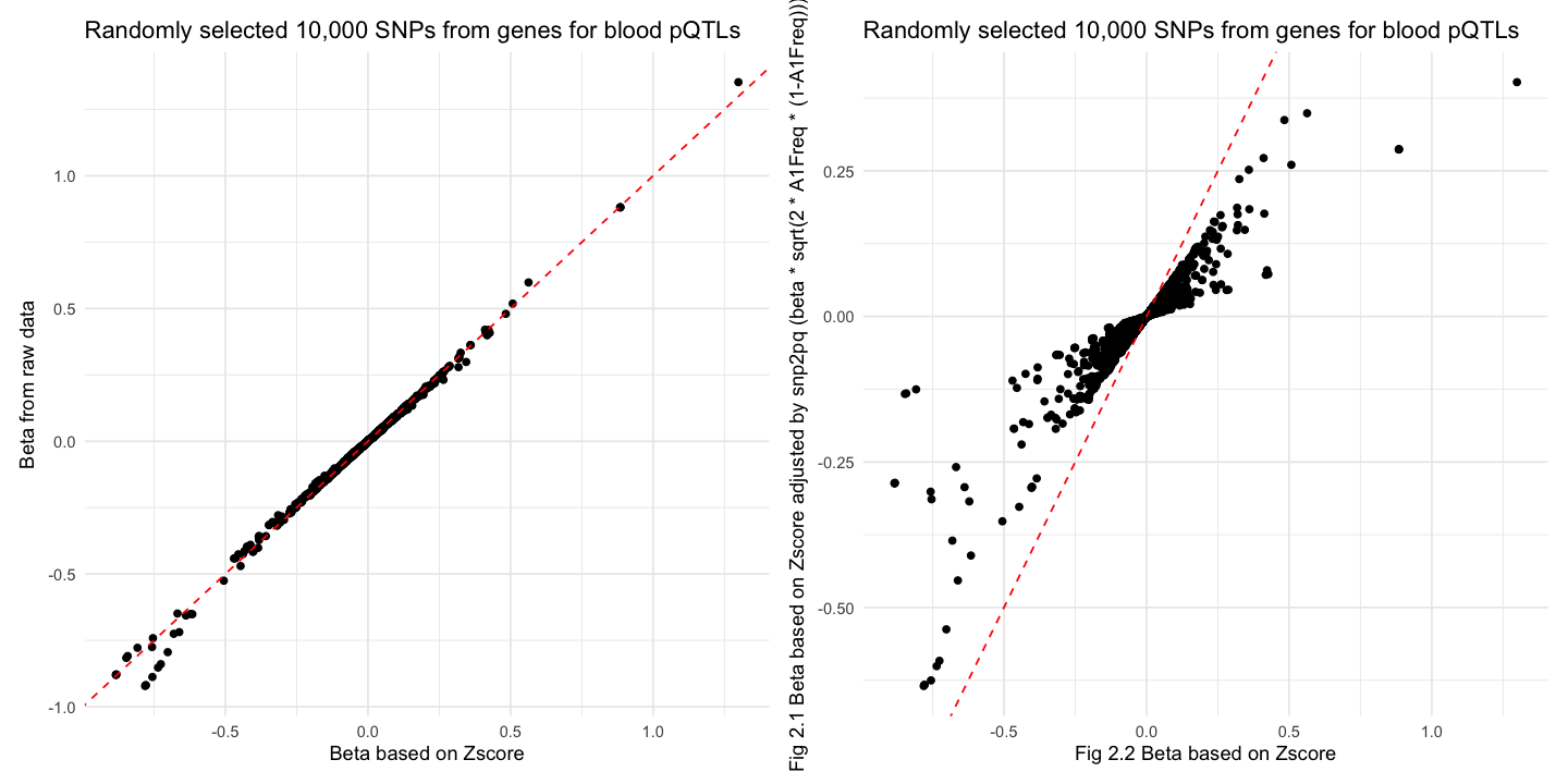
The transformation behavior in blood pQTLs data is highly similar to the simulated results. The systematic bias pattern (negative values shrinking, positive values stretching) remains evident.

############################################
### Brain eQTLs
############################################
library(data.table)
library(tidyverse)
beqtlPath = "~/Downloads/data/xqtl/"
beqtl = fread(paste0(beqtlPath,"QC-HM3-brain-gene16620-eqtl-1086269-cis1M-chr1-22-2025-03-17.query.gz"))
test = beqtl %>% mutate(zz = BETA/SE) %>%
mutate(beta = zz / sqrt(2 * A1Freq * (1-A1Freq) * (N-1 + zz^2)),
       betaScale = BETA * sqrt(2 * A1Freq * (1-A1Freq)),
se = 1 / sqrt(2 * A1Freq * (1-A1Freq) * (N-1 + zz^2))
) %>% slice_sample(n = 10000)
head(test)
options(repr.plot.width = 12, repr.plot.height = 6)
p1 = ggplot(test, aes(x = beta, y = BETA)) +
  geom_point() +
  geom_abline(intercept = 0, slope = 1, linetype = "dashed", color = "red") +
  labs(
    y = "Beta from raw data",
    x = "Beta based on Zscore",
    title = "Randomly selected 10,000 SNPs from genes for brain eQTLs"
  ) + theme_minimal()
p2 =  test  %>%
mutate( betaScale = BETA * sqrt(2 * A1Freq * (1-A1Freq))) %>%
 ggplot( aes(x = beta, y = betaScale)) +
  geom_point() +
  geom_abline(intercept = 0, slope = 1, linetype = "dashed", color = "red") +
  labs(
    y = "Fig 3.1 Beta based on Zscore adjusted by snp2pq (beta * sqrt(2 * A1Freq * (1-A1Freq)))",
    x = "Fig 3.2 Beta based on Zscore",
    title = "Randomly selected 10,000 SNPs from genes for brain eQTLs"
  ) + theme_minimal()
  p1 + p2

print(paste0("correlation between beta and BETA is ", cor(test$beta, test$BETA)))
print(paste0("correlation between beta and betaScale is ", cor(test$beta, test$betaScale)))

A data.table: 6 x 18

GeneID	GeneChr	GeneLength	GenePhyPos	SNPID	SNPChr	SNPPhyPos	A1	A2	A1Freq	BETA	SE	Pvalue	N	zz	beta	betaScale	se
<chr>	<int>	<int>	<int>	<chr>	<int>	<int>	<chr>	<chr>	<dbl>	<dbl>	<dbl>	<dbl>	<int>	<dbl>	<dbl>	<dbl>	<dbl>
ENSG00000143771.12	1	-999	224555860	rs4653593	1	224881970	A	G	0.213115	-0.006912926	0.03710873	0.85221859	2865	-0.1862884	-0.006010617	-0.004003497	0.03226512
ENSG00000146909.8	7	-999	156754138	rs4078489	7	155858530	C	T	0.371585	-0.006239648	0.03607818	0.86269234	2865	-0.1729480	-0.004728891	-0.004264100	0.02734286
ENSG00000254343.2	8	-999	121066430	rs10093792	8	121515110	A	G	0.314208	-0.097312212	0.03977902	0.01443229	2865	-2.4463199	-0.069559050	-0.063883274	0.02843416
ENSG00000272512.1	1	-999	932388	rs2250833	1	1854321	A	G	0.306011	0.044837367	0.03829468	0.24165865	2865	1.1708511	0.033562277	0.029221325	0.02866486
ENSG00000213199.8	7	-999	150747611	rs11984138	7	150300735	A	G	0.224044	-0.004591339	0.03181196	0.88524191	2865	-0.1443274	-0.004573626	-0.002707320	0.03168923
ENSG00000139209.16	12	-999	47192368	rs2465230	12	47324596	T	C	0.423497	-0.087216511	0.03631631	0.01632444	2865	-2.4015800	-0.064155329	-0.060945222	0.02671380

[1] "correlation between beta and BETA is 0.978783611798265"
[1] "correlation between beta and betaScale is 0.931821297460271"

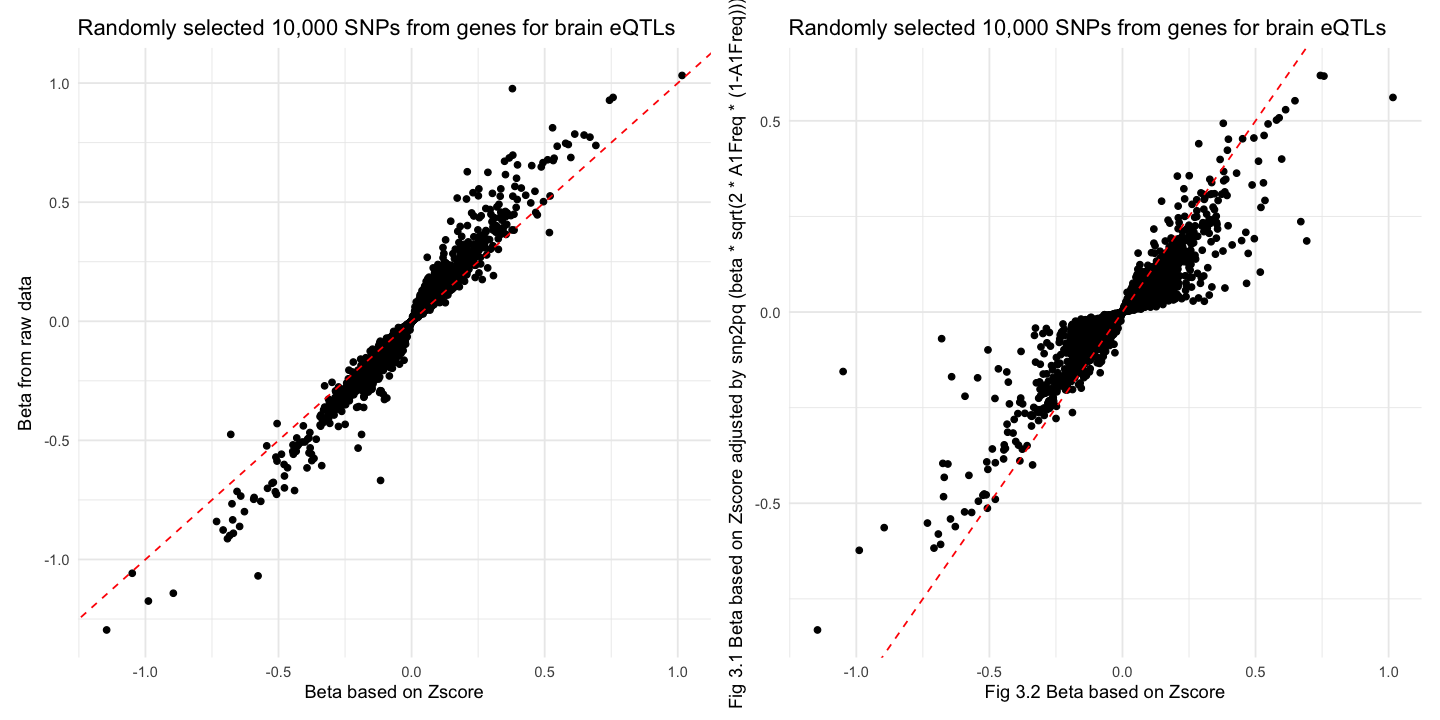
Similar trend was found in brain eQTLs but Fig 3.1 had larger variance since here we use unique total sample size for all eQTLs.

# Extreme effect for snp rs7749880
# /QRISdata/Q4062/softwares/smr/smr --beqtl-summary  BrainMeta_cis_eQTL_chr6 --snp rs7749880 --out myquery --query
# SNP	Chr	BP	A1	A2	Freq	Probe	Probe_Chr	Probe_bp	Gene	Orientation	b	SE	p
# rs7749880	6	58346584	A	G	0.469945	ENSG00000271761.1	6	58229156	AL021368.1	-	-0.137552	0.0222519	6.34526e-10
# rs7749880	6	58346584	A	G	0.469945	ENSG00000215190.9	6	58280066	LINC00680	-	**-3156.06**	2.8288	0

# Cis-sQTL mapping was conducted using FastQTL, testing for associations between genetic variants located within ±1 Mb of 
# each gene’s transcription start site (TSS). The analysis incorporated the covariates detailed in Section 4.1, along with
# 15 PEER factors derived from splicing quantifications (Section 3.5.2) (GTEx Consortium, 2020). 

# FastQTL(Ongen, Halit, et al.(2016)) utilizes normalized gene expression data, covariate matrices, and dosage genotype information
# within a regression framework to identify statistically significant associations between genetic variants and molecular phenotypes,
# thereby uncovering both cis (proximal) and trans (distal) QTLs.