Imputation and adjustment#
Theory underlying the adjustment of sample sizes in GWAS (molQTL) summary statistics#
For a given gene (or protein), we defined \(b_j^{(c)}\) as the molQTL effect for SNP \(j\) with the current sample size and \(b_j^{(t)}\) as that with the target sample size. Under the assumption of normality and unit phenotypic variance, the joint distribution of \(b_j^{(c)}\) and \(b_j^{(t)}\) can be approximated by a bivariate normal distribution.
For each gene, given the marginal effect-size vector \(\mathbf{b}^{(c)}\) and LD matrix \(\mathbf{R}\), the conditional distribution of \(\mathbf{b}^{(t)} \mid \mathbf{b}^{(c)}\) is:
where \(n_c\) and \(n_t\) are the current and target sample sizes for each molQTL within that gene, respectively, with \(\mathbf{b}^{(c)}\) used as a surrogate of the true effect sizes.
Eigen-decomposition with a maximum cut-off of variance explained (\(\rho = 0.995\)) was applied to the LD matrix to generate a pseudo-inverse of \(\mathbf{R}\). The summary statistics under the target sample size were then estimated as:
where \(\mathbf{U}\) and \(\mathbf{\Lambda}\) are matrices of eigenvectors and eigenvalues of the LD matrix \(\mathbf{R}\), and \(\xi_j \sim \mathcal{N}(0, 1)\) is a standard normal random variable for SNP \(j\).
The marginal standard errors (SE) for \(b^{(t)}\) and \(b^{(c)}\) are:
Equivalently, \(\mathrm{SE}^{(t)}\) can be estimated as:
Implementation of method to adjust sample sizes in GWAS (molQTL) summary#
#############################################################
### R demo for adjusting sample sizes in GWAS (molQTL) summary
#############################################################
rm(list = ls())
suppressPackageStartupMessages({
library(tidyverse)
library(data.table)
library(patchwork)
library(latex2exp)
library(cowplot)
})
set.seed(1234)
if (!requireNamespace("SBayesOmics", quietly = TRUE)) {
devtools::install_github("ShouyeLiu/SBayesOmics")
}
library(SBayesOmics)
sumPath = system.file("extdata/summary/", package = "SBayesOmics")
smrIndFileSuffix = "ukbg-chr22-causal-model-50k-ind"
geneLDFile = paste0(sumPath,smrIndFileSuffix)
geneSummaryFile = paste0(sumPath,smrIndFileSuffix)
qtlP50K = downsampleN(geneSummaryFile,geneLDFile,targetN = 50000)
qtlP10K = downsampleN(geneSummaryFile,geneLDFile,targetN = 10000)
qtlP1K = downsampleN(geneSummaryFile,geneLDFile,targetN = 1000)
datPse<- rbind(qtlP50K,qtlP10K,qtlP1K)
############################################################
## specific theme
themeLocal = theme_bw() + theme(axis.text=element_text(size=10,face = "bold"),
axis.title=element_text(size=10,face="bold"),
axis.title.x = element_text(size = 8.5), # Adjust the size as needed
axis.title.y = element_text(size = 8.5),
legend.title=element_text(size=10,face="bold"),
legend.text=element_text(size=10,face = "bold"),
panel.grid.major = element_line(color = "white", linewidth = 0.2),
panel.grid.minor = element_line(color = "white", linewidth = 0.1),
plot.subtitle = element_text(size = 9, face = "bold", hjust = 0.5),
strip.text = element_text(size = 5.5),
aspect.ratio = 1 ,
axis.text.x = element_text(size = 8,angle = 45,hjust = 1),
axis.text.y = element_text(size = 8),
legend.position.inside = c(0.65, 0.12),
legend.background = element_rect(fill = alpha("white", 0.5) )
)
datPse$N = factor(datPse$N)
mycolors = c("#45b787", "#f03f24","black")
##########################################
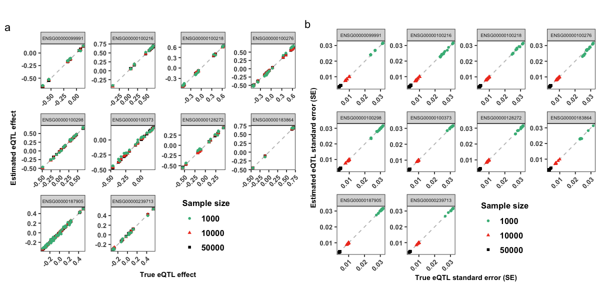
pMBeta = datPse %>% as.data.table() %>%
ggplot(aes(x = betaR,y = betaPse,color = N,shape = N)) +
geom_abline(intercept = 0, slope = 1,linetype = "dashed", color = "grey") +
geom_point(size = 0.9, stroke = 1) +
xlab("True eQTL effect") +
ylab("Estimated eQTL effect") +
scale_fill_manual(values=mycolors) +
scale_color_manual(values=mycolors)+
facet_wrap(~ GeneID,scales = "free") +
themeLocal + # + theme(legend.position = "none") +
labs(color = "Sample size", shape = "Sample size") +
labs(tag = 'a')
pMSe = datPse %>% as.data.table() %>%
ggplot(aes(x = seR,y = sePse,color = N,shape = N )) +
geom_abline(intercept = 0, slope = 1,linetype = "dashed", color = "grey") +
geom_point( size = 0.9,stroke = 1) +
xlab("True eQTL standard error (SE)") +
ylab("Estimated eQTL standard error (SE)") +
scale_fill_manual(values=mycolors) +
scale_color_manual(values=mycolors)+
facet_wrap(~ GeneID,scales = "free") +
themeLocal +
labs(color = "Sample size", shape = "Sample size") +
# guides(color = guide_legend(title = "Sample size")) +
labs(tag = 'b')
fplot <- plot_grid(pMBeta, pMSe, ncol = 2, rel_widths = c(1, 1))
# # Show it
options(repr.plot.width = 10, repr.plot.height = 5) # adjust size
print(fplot)
10 gene low-rank marices have been read.

10 gene low-rank marices have been read.

10 gene low-rank marices have been read.
Citation#
[1] Shouye Liu, Xiaoyu Qian, Yang Wu, Zhili Zheng, Michael E. Goddard, Jian Yang, Peter M. Visscher, Jian Zeng. Transcriptional and translational genetic control in blood contributes significantly to complex trait heritability and polygenic prediction. Preprint available on bioRxiv doi: https://doi.org/10.1101/2025.05.24.25328265